Math 132A
Introduction to Inference
What is statistical inference?
Goal: Create a mathematical model for some random variable, or for an association between two or more random variables.
This may involve:
Creating a new model
Evaluating an existing model
Model for a random variable: A distribution with some parameters.
Model for an association between random variables: It’s complicated.
Population
-
The random variable(s) is (are) tied to some “population”:
- All patients in some hospital that have certain disease
- All patients in the world that currently have certain disease
- All potential patients in the world that currently have certain disease, or had the disease in the past, or will have the disease in the future
- All plants of certain species in a given forest.
- All plants of certain species, in the past, now, and in the future
- All adults currently living in the US
- All current, past and future adults in the US
We then talk about the population distribution, the population parameter, and a model of the population.
Examples
-
Population: All potential patients in the world that currently have certain disease, or had the disease in the past, or will have the disease in the future
- Variable: Length of the incubation period for the disease.
- Variable: Were the patients given some specific treatment?
- Variable: Patient’s age.
-
Population: All plants of certain species in a given forest
- Varaible: Height of each plant.
- Varaible: Does the plant have certain genetic mutation.
Unreasonably optimistic goal
By looking at a sample, figure out exactly what model to use for the population variable.
That means complete description of the distribution, including the exact values of all the parameters.
We only have a sample of the values, that’s not going to be enough.
Samples vary!!!
Realistic goals
Figure out something about one of the parameters, or
Figure out something about the way the variable is distributed.
Perhaps we already have some idea about the type of the distribution, can we learn something about its parameter(s)?
What can we learn from a sample?
Simplest case: The variable can be modeled by a Bernoulli distribution with some (unknown) probability of success \(p\).
Certain (unknown) proportion \(p\) of residents of a city are infected with some virus.
Certain (unknown) proportion \(p\) of voters will vote for a specific candidate.
Certain (unknown) proportion \(p\) of gadgets made in a factory are faulty.
In a sample of \(n\) independent value, the number of successes \(x\) will be a \(\operatorname{Binom}(n, p)\) random variable.
Sample Statistic
In a sample of \(n\) independent value, the number of successes \(x\) will be a \(\operatorname{Binom}(n, p)\) random variable.
We say that \(x\) is a sample statistic, and its sampling distribution is \(\operatorname{Binom}(n, p)\).
Another, better, sample statistic is the sample proportion of successes: \[\widehat{p} = \frac{x}{n}\]
\(\widehat p\) is a point estimate for \(p\).
Sampling Distribution of \(\widehat p\)
Sampling distribution of \(x\) is \(\operatorname{Binom}(n, p)\).
The mean of \(x\) is \(np\), the variance of \(x\) is \(np(1-p)\), and the standard error of \(x\) is \(\sqrt{np(1-p)}\).
If \(np\) and \(n(1-p)\) are large enough, we can approximate the sampling distribution of \(x\) by \(\displaystyle\operatorname{N}\left(np, \sqrt{np(1-p)}\right)\).
What is the mean, variance, and standard error of \(\widehat{p}\)?
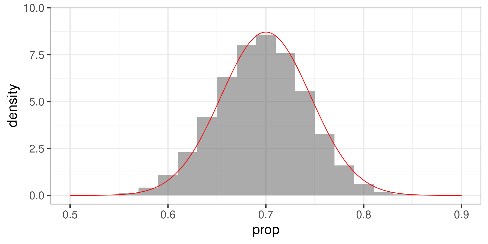
The sampling distribution of \(\widehat{p}\) can be approximated by \(\displaystyle\operatorname{N}\left(p, \sqrt{\frac{p(1-p)}{n}}\right)\).
Central Limit Theorem for Proportions
Samples consists of \(n\) independent values of the same Bernoulli variable with probability of success \(p\).
The success-failure condition: Both \(np\) and \(n(1-p)\) are sufficiently large.
Then the sample proportions \(\widehat{p}\) are approximately normally distributed with mean \(p\) and standard error \[\sqrt{\frac{p(1-p)}{n}}\]
Example
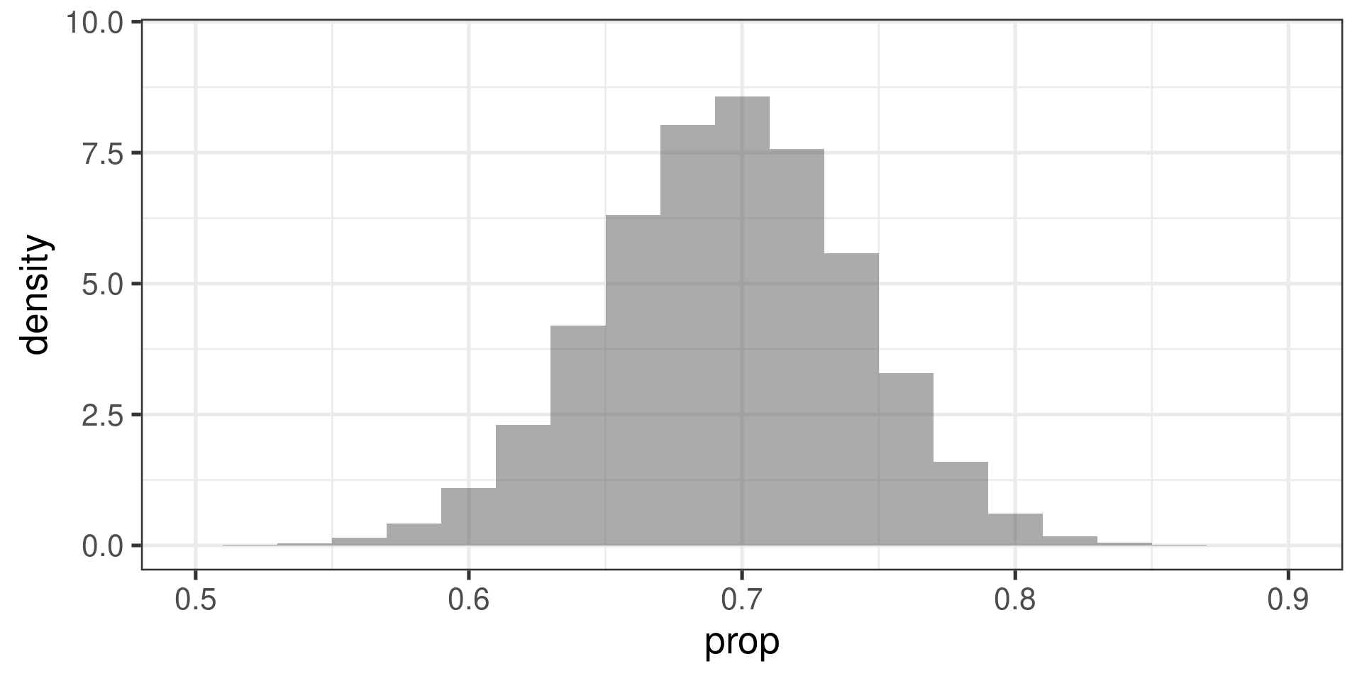
Population: \(p = 0.7\)
Sample size: \(n = 100\)
Sampling distribution for \(\widehat{p}\):
How it looks like
Using the CLT to calculate probabilities
A sample of size \(n = 100\) is drawn from a population in which \(p = .7\).
- Calculate the probability that \(\widehat{p} \le .75\).
- Calculate the probability that \(\widehat{p} \ge .67\).
- Calculate the probability that \(.67 \le \widehat{p} \le .75\).