tally(~Diabetes, data = nhanes.samp.adult, margin = TRUE)Diabetes
No Yes Total
122 13 135 Confidence Intervals Examples
What proportion of Americans have diabetes?
We used the nhanes.samp.adult data set, which includes the Diabetes variable:
tally(~Diabetes, data = nhanes.samp.adult, margin = TRUE)Diabetes
No Yes Total
122 13 135 The sample proportion of subjects with diabetes is \[\hat{p} = 0.0962963.\]
What does this tell us about the population proportion?
According to this sample, what are the plausible values of the population proportion?
Get the bootstrap distribution:
do(10000) * tally(~Diabetes, data = resample(nhanes.samp.adult),
                  format = "proportion") -> boots
Visualize it
gf_histogram(~Yes, data = boots)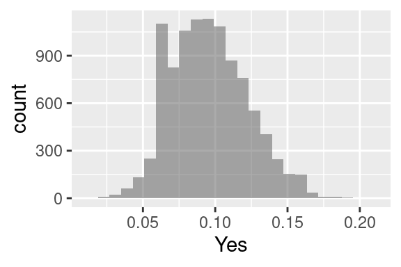
Get the 95% CI:
qdata(~Yes, c(0.025, 0.975), data = boots) 2.5% 97.5%
0.05185185 0.14814815 We are 95% confident that the interval between 0.052 and 0.148 contains the true proportion of the US adults who have diabetes.
According to the CLT for proportions, the sampling distribution of sample proportions is approximately \[N\left(p, \sqrt{\frac{pq}{n}}\right).\]
It is contingent on the success-failure condition: \(np\) and \(nq\) must both be at least 10.
For confidence interval, we are sampling from the bootstrap population.
That is a fake population that is perfectly represented by the sample.
In this population, \(p\) is \(\hat{p}\) and \(q\) is \(\hat{q}\).
\(n\hat{p}\) is the actual number of successes in the sample.
\(n\hat{q}\) is the actual number of failures in the sample.
According to the CLT for proportions:
95% of all values of a standard normal distribution are between \(-1.96\) and \(1.96\).
95% of all values of \(N(0.0962963, 0.0253893)\) are between \[0.0962963 - 1.96\cdot 0.0253893 = 0.0465332\] and \[0.0962963 + 1.96\cdot 0.0253893 = 0.1460593.\]
Using R:
We are 95% confident that the interval between 0.047 and 0.146 contains the true proportion of the US adults who have diabetes.
Bootstrapping:
do(10000) * tally(~Diabetes, data = resample(nhanes.samp.adult),
                  format = "proportion") -> boots

qdata(~Yes, c(0.025, 0.975), data = boots)
2.5% 97.5%
0.05185185 0.14814815 Using the same data set, we also found a confidence interval for the mean height of US adults. Let’s look at this example again.
favstats(~Height, data = nhanes.samp.adult) min Q1 median Q3 max mean sd n missing
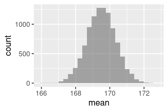
140 162.55 168.5 177.8 191.3 169.4874 9.949473 135 0We will find a 98% confidence interval for the population mean. We will use both bootstrapping and the Central Limit Theorem.
We are 98% confident that the interval between 167.52 cm and 171.45 cm contains the true mean height of all US adults.
favstats(~Height, data = nhanes.samp.adult) min Q1 median Q3 max mean sd n missing
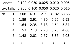
140 162.55 168.5 177.8 191.3 169.4874 9.949473 135 0Interval: \((\overline{x} - t^\star\cdot SE,\overline{x} + t^\star\cdot SE) = (169.4874074 - 2.0161903, 169.4874074 + 2.0161903) = (167.4712171, 171.5035977)\)
We are 98% confident that the interval between 167.47 cm and 171.5 cm contains the true mean height of all US adults.
We need to know \(\alpha = 1 - L\).
Left or lower CI: the area to the left of \(z^\star\) is \(\alpha\).
With \(\alpha = 0.05\) (\(95\)% CI):
qnorm(0.05)[1] -1.644854Right or upper CI: the area to the left of \(z^\star\) is \(1 - \alpha\).
With \(\alpha = 0.05\) (\(95\)% CI):
qnorm(0.95)[1] 1.644854Two-sided CI: the area to the left of \(z^\star\) is \(1 - \alpha/2\).
With \(\alpha = 0.05\) (\(95\)% CI):
qnorm(0.975)[1] 1.959964We need \(\alpha = 1 - L\) and \(n\) for degrees of freedom. \(df = n - 1\)
Left or lower CI: the area to the left of \(t^\star\) is \(\alpha\).
With \(\alpha = 0.05\) (\(95\)% CI) and \(n = 25\):
qt(0.05, df = 24)[1] -1.710882Right or upper CI: the area to the left of \(t^\star\) is \(1 - \alpha\).
With \(\alpha = 0.05\) (\(95\)% CI) and \(n = 25\):
qt(0.95, df = 24)[1] 1.710882Two-sided CI: the area to the left of \(t^\star\) is \(1 - \alpha/2\).
With \(\alpha = 0.05\) (\(95\)% CI) and \(n = 25\):
qt(0.975, df = 24)[1] 2.063899Make the \(t^\star\) negative for left (lower) interval.
In some places, rocks found in fields may contain geodes in them. In a sample of 25 rocks collected from a field, 11 of them contained a geode. Use this information to find a 75% confidence interval estimating the proportion of rocks that contain geodes in the field.
In some places, it is possible to find pieces of rare natural glass called tektites. It is known that sizes of tektites are approximately normally distributed. A sample of 16 tektites collected from a field has a mean weight of 12 grams, with standard deviation 3 grams. Use this information to find a 90% confidence interval estimating the mean weight of tektites in the field.