do(10000) * tally(~Diabetes, data = resample(nhanes.samp.adult),
format = "proportion") -> bootsMath 132A
Confidence Intervals
What is statistical inference?
Goal: Create or evaluate a mathematical model for some random variable(s), using a sample of its (their) values.
Model for a random variable: A distribution with some parameters.
Basic methods of inference
We have a model that we think may work, and we want to test it against our data.
We want to see whether the model is consistent with the data.
Use a sample to find an estimate for one parameter of the model.
Requires no previous knowledge of the parameter, although we may have to make some assumptions about the model.
Point estimates
We have one sample, and we want to use it to estimate a population parameter.
Suppose I use the sample mean to estimate the population mean.
That’s called a point estimate
- Because of sampling variation, the point estimate is likely not exactly right.
We think that most of the time the estimate will be pretty good.
What does most of the time mean?
What does pretty good mean?
Sampling Error
There is often going to be some difference between the sample statistic and the population parameter.
This is called a sampling error.
How big can this error get?
General principle: the distribution of the sampling error has the same shape as the sampling distribution of the statistic, but is centered at 0.
Also, the sampling distribution of the statistic will have approximately the same shape as the bootstrap distribution.
Is the Sampling Error Large?
We saw that bootstrap distributions are generally bell shaped.
Most samples will have small sampling error.
There will be a few samples with large sampling error.
We do not know if our sample has small or large sampling error.
-
What we can ask is:
Assuming our sample is one of the good ones, how far from our sample statistic can the population parameter be?
This is called the margin of error.
Confidence Level
- We need to decide which sampling errors are small and which are large.
- In other words, we need to decide which samples are the good samples.
- There are different ways to do that.
- One that is often used is a confidence level:
- We pick some large percentage, let’s say 95%.
- Then we pick the 95% of samples with the smallest sampling error. These will be considered good.
- The remaining 5% will be “bad”.
- This percentage is called the confidence level, denoted \(L\).
Confidence Intervals
- We have one sample.
- Again, we do not know whether it is one of the good samples or not!
- Assuming it is a good sample, how far can the population parameter be from the sample statistic?
- We know that the sampling error distribution has similar shape to the bootstrap distribution.
- Let’s pick the middle 95% of the bootstrap samples, and see which range will they give us.
- If our sample is one of the 95% good ones, then this range should contain the population parameter!
- This is called a 95% confidence interval
- This gives us a plausible range of values for the population parameter, assuming our sample is good.
Quantiles
How do we pick the middle 95% (or whatever other confidence level we want) of the samples?
- It is done using quantiles
- Quantiles are a generalization of quartiles:
- The first quartile separates the lowest 1/4 of the data from the rest.
- The third quartile separates the lowest 3/4 of the data from the rest.
- Given a fraction \(p\) between 0 and 1, the \(p\) quantile is a number that separates the lowest \(p\) of the data from the rest.
- So the first quartile is 1/4 quantile, or 0.25 quantile.
- The second quartile is 3/4 quantile, or 0.75 quantile.
- The 0.025 quantile separates the lowest 2.5% from the rest.
- The 0.975 quantile separates the highest 2.5% from the rest.
Example
-
Get the bootstrap distribution:
-
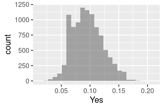
Visualize it
gf_histogram(~Yes, data = boots)![]()
-
Get the 95% CI:
qdata(~Yes, c(0.025, 0.975), data = boots)2.5% 97.5% 0.05185185 0.14814815
Conclusion
We are 95% confident that the interval between 0.052 and 0.148 contains the true proportion of the US adults who have diabetes.
Different Confidence Level
If we instead choose \(L = 90\%\):
qdata(~Yes, c(0.05, 0.95), data = boots) 5% 95%
0.05925926 0.14074074 We are 90% confident that the interval between 0.059 and 0.141 contains the true proportion of the US adults who have diabetes.
Let’s try \(L = 80\%\):
qdata(~Yes, c(0.1, 0.9), data = boots) 10% 90%
0.06666667 0.13333333 We are 80% confident that the interval between 0.067 and 0.133 contains the true proportion of the US adults who have diabetes.
The Confidence Level Interpretation
If this range is narrow, we have a sharp estimate.
If this range is wide, we have an estimate that is not so good.
The correct interpretation:
The method illustrated for computing a 95% confidence interval will produce an interval that (on average) contains the true population mean for 95 samples out of 100.
The remaining 5 samples out of 100 will be “incorrect”, that is, it will not contain the population mean.
Unfortunately, we do not know whether a particular interval contains the population mean.
Accuracy vs. Precision
Accuracy is given by the confidence level. This tells you how likely you are to “hit the target”.
Precision is determined by the width of the interval. This tells you how precisely is the target determined when you hit it.
If you want to increase the accuracy, you have to decrease the precision, and vice versa.