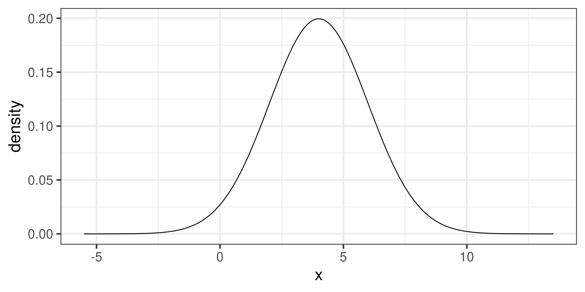
gf_dist("norm", params=c(mean = 4, sd = 2))Math 132A
Central Limit Theorem
Central Limit Theorem (part 1)
When sampling from a population that is normally distributed with mean \(\mu\) and standard deviation \(\sigma\):
- The sample means are also normally distributed…
- … with the same mean \(\mu\)…
- … and standard deviation \[\sigma_{\bar{X}} = \frac{\sigma}{\sqrt{n}}\] where \(n\) is the sample size.
Central Limit Theorem (part 2)
When sampling from any population with mean (expected value) \(\mu\) and finite standard deviation \(\sigma\), then for large enough samples:
- The sample means are approximately normally distributed…
- … with the same mean \(\mu\)…
- … and standard deviation \[\sigma_{\bar{X}} = \frac{\sigma}{\sqrt{n}}\] where \(n\) is the sample size.
- The approximation gets better as the sample size increases.
What does this mean?
With a large sample, the sample mean is likely to be a pretty good estimate of the population mean.
Even if we know nothing about the population distribution, we do know (approximately) the distribution of the sample means, so we can create a mathematical model of the sampling distribution.
The normal distribution
- Special shape of the density curve (kind of like a bell)
- Symmetric, centered around a specific number (called the mean, denoted \(\mu\))
- The “width” of the “bell” depends on the spread of the distribution (the amount of uncertainty), and is usually determined by the standard deviation, denoted by \(\sigma\).
- Variable \(X\) having a normal distribution with given \(\mu\) and \(\sigma\) is denoted at \(X \sim N(\mu, \sigma)\).
The normal distribution
The normal distribution
gf_dist("norm", params=c(mean = 4, sd = 2)) |>
    gf_dist("norm", mean = 4, sd = 3, color="red")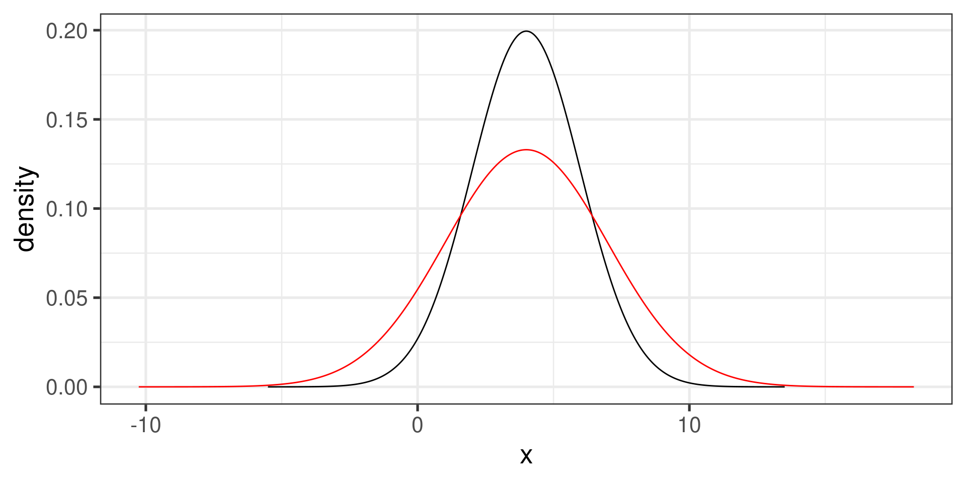
Meaning of Standard Deviation
Empirical Rule for normal distribution:
approximately 68% of the values are within 1 SD of the mean
approximately 95% of the values are within 2 SDs of the mean
approximately 99.7% of the values are within 3 SDs of the mean

68-95-99.7
A Normal Example
The distribution of test scores on the SAT and the ACT are both nearly normal.
Suppose that one student scores an 1800 on the SAT (Student A) and another student scores a 24 on the ACT (Student B). Which student performed better?
A Normal Example

Standard Normal Distribution
The standard normal distribution is defined as a normal distribution with mean 0 and variance 1. It is often denoted as \(Z \sim N(0, 1)\).
Any normal random variable \(X\) can be transformed into a standard normal random variable \(Z\).
\[Z = \dfrac{X - \mu}{\sigma} \qquad X = \mu + Z\sigma\]
A Normal Example…
SAT scores are \(N(1500, 300)\). ACT scores are \(N(21,5)\).
\(x_A\) represents the score of Student A; \(x_B\) represents the score of Student B.
\[z_{A} = \frac{x_{A} - \mu_{SAT}}{\sigma_{SAT}} = \frac{1800-1500}{300} = 1 \]
\[z_{B} = \frac{x_{B} - \mu_{ACT}}{\sigma_{ACT}} = \frac{24 - 21}{5} = 0.6\]
Calculating Normal Probabilities (I)
What is the percentile rank for a student who scores an 1800 on the SAT for a year in which the scores are \(N(1500, 300)\)?
-
Calculate a \(Z\)-score. If \(X\) is a normal random variable with mean \(\mu\) and standard deviation \(\sigma\), \[Z = \frac{X - \mu}{\sigma}, \] is a standard normal random variable (\(\mu = 0\), \(\sigma =1\)).
(1800 - 1500)/300[1] 1 -
Find the normal probability in one of the tables, or let
Rdo the work:pnorm(z)calculates the area (i.e., probability) to the left of \(z\)pnorm(1)[1] 0.8413447
Alternatively, let R do all the work …
What is the percentile rank for a student who scores an 1800 on the SAT for a year in which the scores are \(N(1500, 300)\)?
pnorm(1800, mean = 1500, sd = 300)[1] 0.8413447Calculating Normal Probabilities (II)
Which score on the SAT would put a student in the 99\(^{th}\) percentile?
-
Identify the \(Z\)-value from the table or using
R:qnorm(p)calculates the value \(z\) such that for a standard normal variable \(Z\), \(p = P(Z \leq z)\).qnorm(0.99)gives us 2.326348, or approximately 2.33. -
Calculate the score, \(X\). If \(Z\) is distributed standard Normal, then \[X = \sigma Z + \mu\] is Normal with mean \(\mu\) and standard deviation \(\sigma\).
\[X = \sigma Z + \mu = 300(2.33) + 1500 = 2199\]
Alternatively, let R do the work …
Which score on the SAT would put a student in the 99\(^{th}\) percentile?
qnorm(0.99, mean = 1500, sd = 300)[1] 2197.904The q in qnorm stands for quantile.
Another example
Find the probability that \(X \ge 17.5\) if \(X \sim N(13, 2.5)\)
-
Calculate the \(z\)-score:
\[z = \frac{17.5 - 13}{2.5} = 1.8\]
Now we need to find the area to the right of 1.8 under the standard normal curve.
The original curve
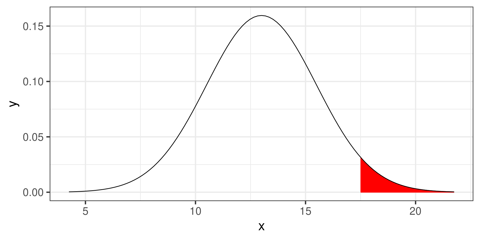
Area to the right of 17.5.
The standard normal curve
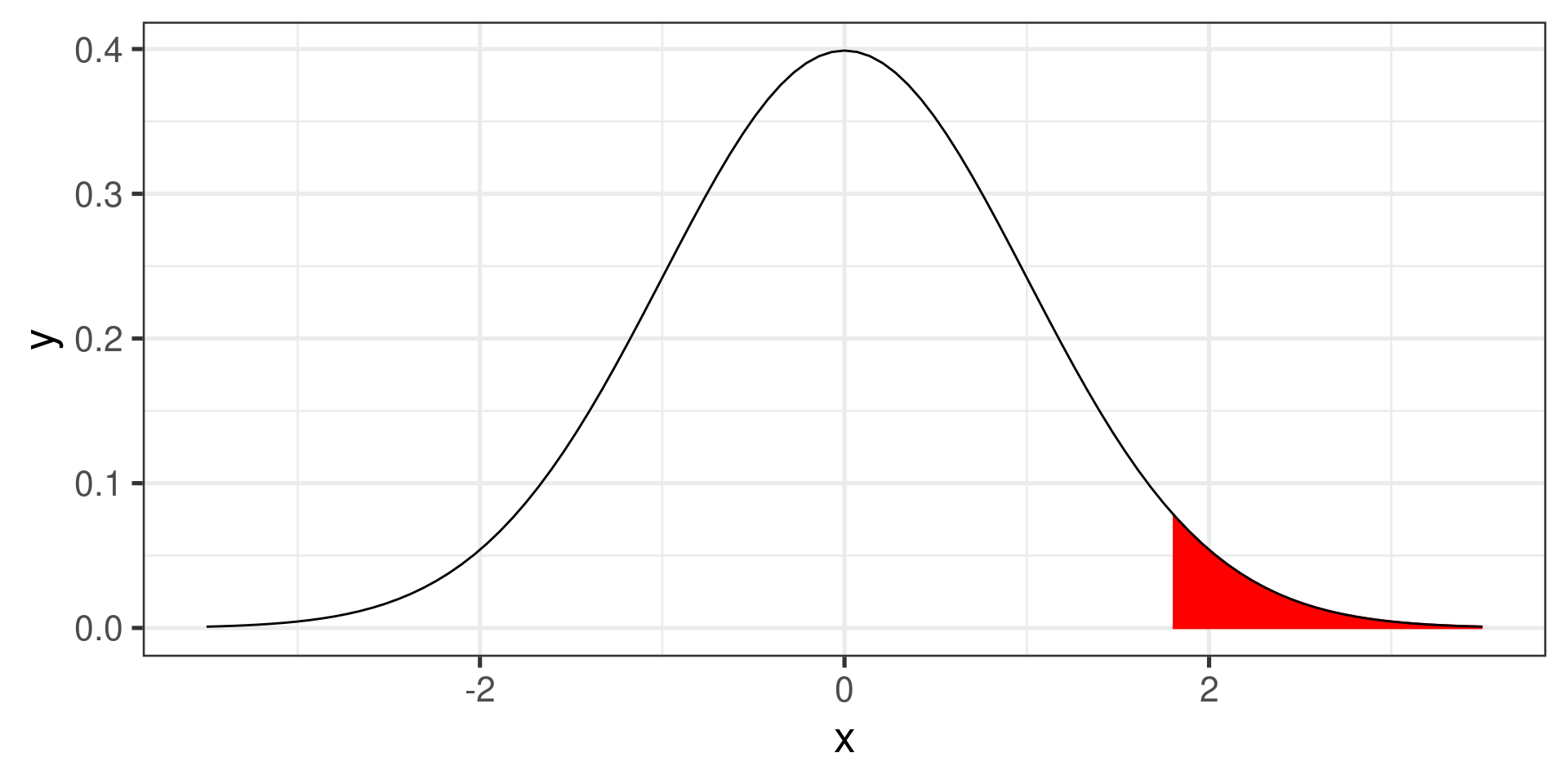
Area to the right of 1.8.
Wrong area
- Both R and the tables give you area to the left of a given \(z\)-score!
Like this:
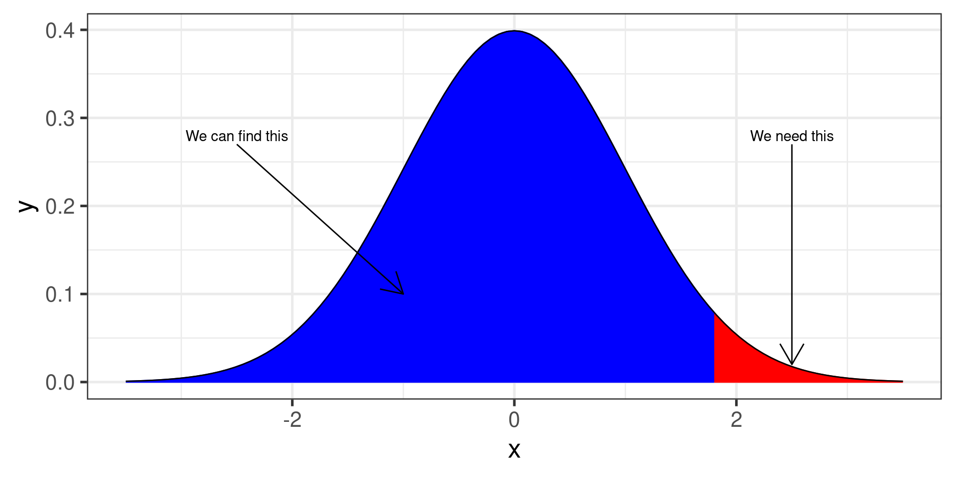
Subtraction
The total area under the normal curve is always 1.
-
All we need to do is subtract:
area to the right = 1 - area to the left
Finally, we can find the area to the right of 1.8.
1 - pnorm(1.8)[1] 0.03593032pnorm(1.8, lower.tail=FALSE)[1] 0.03593032